From Autoencoders to VQ-VAE
: An intuitive guide to understanding Autoencoders
Table of Contents
Symbol Glossary
| Symbol | Meaning |
|---|---|
| $D$ | The Dataset $D$ contains n data samples |
| $x$ | One data point from dataset (a single example, like an image), $ x \in D $ |
| $x^{(i)}$ | The $i$-th data point, a vector in $\mathbb{R}^d$, i.e., $x^{(i)} \in \mathbb{R}^d$ |
| $x’$ | Reconstructed version of $x$ |
| $\tilde{x}$ | Corrupted version of $x$ |
| $z$ | Latent variable (vector) unobserved “cause” of $x$ |
| $a^l_j$ | Activation function for $j^{\text{th}}$ neuron in hidden layer $l$ |
| $g_\phi(.)$ | Encoder with parameter $\phi$ |
| $f_\theta(.)$ | Decoder with parameter $\theta$ |
| $p_\theta(x, z)$ | Joint distribution of $x$ and $z$ under model parameters $\theta$ |
| $p_\theta(x \mid z)$ | Likelihood the decoder network |
| $p(z)$ | Prior distribution of latent variables (often $\mathcal{N}(0, I)$) |
| $p_\theta(z \mid x)$ | True posterior how likely a latent $z$ explains $x$ |
| $q_\phi(z \mid x)$ | Approximate posterior (encoder) |
| $\mathbb{E}_q[\cdot]$ | Expectation under $q$ |
| $\mathrm{KL}(q \Vert p)$ | Kullback–Leibler divergence |
| $\epsilon$ | Random noise variable used in reparameterization |
| $\nabla_\theta, \nabla_\phi$ | Gradients wrt decoder / encoder parameters |
Autoencoder
Autoencoder is an unsupervised neural network that learns to reconstruct its input by approximating the identity function, while simultaneously compressing the data into a lower-dimensional latent space to discover a more efficient internal representation. It consists of two parts an encoder that maps the input to the latent space, and a decoder that reconstructs the input from the latent code.
\[\mathbf{x \xrightarrow{\text{encoder}} z \xrightarrow{\text{decoder}} {x'}.}\]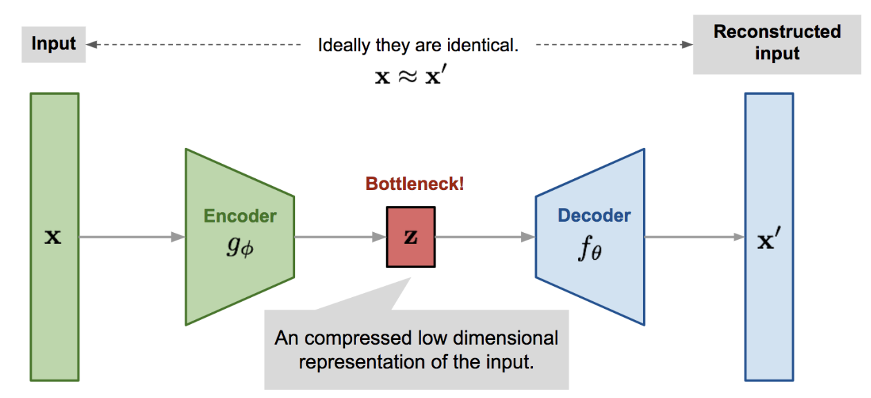
Figure 1: Illustration of Autoencoder model architecture.
For an input $x$, the encoder function $g_\phi(.)$ learns to output a latent code $z$, such that $z = g_\phi(x)$. The decoder $f_\theta(.)$ reconstructes the input as, $ x’= f_\theta(z) = f_\theta(g_\phi(x))$
The parametera $\phi,\theta$ are learned together to reconstruct the datasample. Various metrics can quantify the the difference between the two vectors, such as:
-
Mean Squared Error (MSE) Loss: \(\mathbf{\mathcal{L}_{\text{AE}}(\phi, \theta) = \frac{1}{n} \sum_{i=1}^n (x^i - f_\theta(g_\phi(x^i)))^2}\)
-
Cross Entropy Loss: \(\mathbf{\mathcal{L}_{\text{AE}}(\phi, \theta) = - \frac{1}{n} \sum_{i=1}^n \sum_{j=1}^d x^i_j \log f_\theta(g_\phi(x^i))_j}\)
Denoising Autoencoder
Since the autoencoder learns to reconstruct its input directly, it risks simply copying the input without extracting meaningful structure. Denoising Autoencoders (DEA) Vincent et al. 2008. overcome this by intentionally corrupting the input with partial noise. This forces the network to learn robust, high-level features that are invariant to noise.
More formally, given a data sample $ x $, we apply a stochastic corruption process to get a noisy version \(\tilde{x} \sim \mathcal{M_D}(\cdot | x)\) The encoder then maps this corrupted input to a latent representation:
\[\mathbf{z} = g_\phi(\tilde{x})\]The decoder then reconstructs the original (clean) data sample $x$, from the input latent code:
\[\mathbf{x'} = f_\theta(z) = f_\theta(g_\phi(\tilde{x}))\]So, the model learns to approximate the mapping:
\[\tilde{x} \xrightarrow{\text{encoder}} z \xrightarrow{\text{decoder}} x' \approx x.\]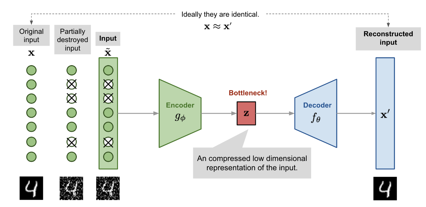
Figure 2: Illustration of denoising autoencoder model architecture.
Sparse Autoencoders
A Sparse Autoencoder (SAE) applies a sparsity constraint on the hidden layer activations to prevent overfitting, encourage feature selectivity, and learn robust representations.
Instead of allowing all neurons to be active for every input, it encourages only a few neurons to activate at once, forcing the model to distribute information more meaningfully across neurons.
A neuron is said to be active if its activation is close to 1 (e.g., in sigmoid, ReLU etc.), and inactive if close to 0. Sparse autoencoders aim to make most hidden neurons inactive for a given input.
Let:
- $ \mathbf{x} \in \mathbb{R}^d $: input vector
- $ \mathbf{z} = g_\phi(\mathbf{x}) \in \mathbb{R}^{d_z} $: hidden (latent) representation
- $ \mathbf{x}’ = f_\theta(\mathbf{z}) \in \mathbb{R}^d $: reconstructed output
We aim to minimize the total loss: \(\mathcal{L}_{\text{SAE}} = \underbrace{\mathcal{L}_{\text{recon}}}_{\text{Reconstruction Loss}} + \underbrace{\lambda \cdot \Omega_{\text{sparse}}}_{\text{Sparsity Penalty}}\)
Sparsity helps discover localized, interpretable features by encouraging the model to activate only a small subset of neurons for any given input. This selective activation means each neuron specializes in detecting specific patterns or features, such as edges in images or particular word groups in text, rather than responding broadly to many inputs. As a result, the learned representations become more focused and disentangled, making it easier to interpret what each neuron encodes, and improving robustness and generalization. Olshausen & Field (1996), Lee et al. (2007).
Reconstruction Loss
For real-valued inputs, we typically use MSE loss:
\[\mathbf{\mathcal{L}_{\text{recon}} = \frac{1}{n} \sum_{i=1}^n \left\| \mathbf{x}^{(i)} - f_\theta(g_\phi(\mathbf{x}^{(i)})) \right\|^2}\]For binary inputs or sigmoid outputs, use cross-entropy:
\[\mathbf{\mathcal{L}_{\text{recon}} = -\frac{1}{n} \sum_{i=1}^n \sum_{j=1}^d \left[ x^{(i)}_j \log x^{\prime(i)}_j + (1 - x^{(i)}_j) \log (1 - x^{\prime(i)}_j) \right]}\]Sparsity Constraint with KL Divergence
Let’s say there are $\mathbf{m}$ neurons in the $\mathbf{l}$-th hidden layer, and the activation function for the $\mathbf{j}$-th neuron in this layer is labelled as $a_j^{(l)}(.)$, $j$ = {$1,2,…..,m$} .
The fraction of activation of this neuron is expected to be a small number $\rho$, known as the sparsity parameter; a common configuration is $\rho = 0.05$.
Mathematically, the average activation of neuron $j$ in layer $l$ is:
\[\hat{\rho}_j = \frac{1}{n} \sum_{i=1}^n a_j^{(l)}(\mathbf{x}^{(i)}) \approx \rho\]To enforce sparsity, we add a penalty term to the loss function using the KL divergence between the desired sparsity $\rho$ and the average activation $\hat{\rho}_j$:
\[\mathrm{KL}(\rho \, \| \, \hat{\rho}_j) = \rho \log \frac{\rho}{\hat{\rho}_j} + (1-\rho) \log \frac{1-\rho}{1-\hat{\rho}_j}\]The overall sparsity penalty across all neurons in the layer is:
\[\Omega_{\text{sparse}} = \sum_{j=1}^m \mathrm{KL}(\rho \, \| \, \hat{\rho}_j)\]Finally, the sparse autoencoder loss function becomes:
\[\boxed{ \mathcal{L}_{\text{SAE}}(\phi, \theta) = \mathcal{L}_{\text{recon}} + \lambda \sum_{j=1}^m \mathrm{KL}(\rho \, \| \, \hat{\rho}_j) }\]This penalty grows rapidly when $ \hat{\rho}_j \gg \rho $, discouraging high activation.
where $\lambda$ controls the weight of the sparsity penalty.
Why KL-Divergence?
KL divergence measures how much each neuron’s average activation deviates from a small sparsity target. By penalizing this difference, it encourages most neurons to stay inactive, enforcing sparsity. This helps the model learn more efficient and interpretable features.
Contractive Autoencoder (CAE)
A Contractive Autoencoder learns to reconstruct its input while encouraging local invariance in its latent representation. It does this by penalizing the sensitivity of the encoder to small input perturbations, effectively encouraging the model to produce similar latent representations for nearby inputs. This contraction of the latent space around the data manifold enhances the robustness and generalization of the learned features.
This property is enforced by adding a regularization term to the loss function: the Frobenius norm of the Jacobian of the encoder’s output with respect to its input. This penalizes the encoder’s sensitivity to small changes in the input, encouraging locally invariant representations.
Standard autoencoders may overfit to the input data, learning representations that are not robust to small input perturbations. CAEs address this by explicitly encouraging the encoder’s output to change minimally with small changes in the input. This leads to smoother and more stable representations.
Let:
- $ x \in \mathbb{R}^d $: input data point
- $ z = g_\phi(x) $: encoded latent representation
- $ x’ = f_\theta(z) = f_\theta(g_\phi(x)) $: reconstruction
- $ \phi, \theta $: encoder and decoder parameters
- $ h = g_\phi(x) \in \mathbb{R}^m $: hidden layer activation
- $ \lambda $: regularization coefficient
The CAE loss is:
\[\mathcal{L}_{\text{CAE}}(x, x') = \underbrace{\|x - x'\|^2}_{\text{Reconstruction Loss}} + \lambda \underbrace{\left\| \frac{\partial h}{\partial x} \right\|_F^2}_{\text{Contractive Penalty}}\]Where:
- $ \left| \cdot \right|_F $: Frobenius norm (i.e., the square root of the sum of squared entries of the Jacobian matrix)
- $ \frac{\partial h}{\partial x} \in \mathbb{R}^{m \times d} $: Jacobian matrix of the encoder’s output with respect to the input
This contractive penalty ensures that the encoder is less sensitive to input changes, pushing representations to lie on a low-dimensional manifold.
Jacobian of Sigmoid Activation
Assuming a sigmoid activation $ h_j(x) = \sigma(W_j x + b_j) $, where $ \sigma(z) = \frac{1}{1 + e^{-z}} $, the partial derivative for each hidden unit is:
\[\frac{\partial h_j}{\partial x} = h_j(x) \cdot (1 - h_j(x)) \cdot W_j\]Thus, the contractive penalty becomes:
\[\left\| \frac{\partial h}{\partial x} \right\|_F^2 = \sum_{j=1}^{m} \left( h_j(x)(1 - h_j(x)) \right)^2 \cdot \|W_j\|^2\]This term penalizes high-weight directions and high curvature in the latent space, effectively smoothing the learned features.
Variational Autoencoder (VAE)
A regular autoencoder learns a mapping:
\[x \xrightarrow{\text{encoder}} z \xrightarrow{\text{decoder}} {x'}.\]It minimizes a reconstruction loss like:
\[\mathcal{L}_{\text{AE}} = \|x - \hat{x}\|^2.\]But this setup has no constraint on what the latent codes $z$ look like.
They could lie anywhere — forming an irregular, “holey” latent space.
So if you sample a random $z \sim \mathcal{N}(0, I)$ and decode it, it probably doesn’t correspond to any real $x$ the network has seen.
In other words, autoencoders compress but don’t truly model data.
The Variational Autoencoder (VAE) changes that.
The idea of Variational Autoencoder (Kingma & Welling, 2014), is deeply rooted in the methods of variational bayesian and graphical model.
-
Instead of encoding an input $ x $ to a single latent vector $ z $, we encode it to a distribution over possible $ z $’s:
$ q_\phi(z \mid x) = \mathcal{N}(\mu_\phi(x), \sigma_\phi(x)^2 I) $. -
We then sample from this distribution to get a latent code and pass it to a decoder to reconstruct $ x $.
-
The goal is twofold:
- Learn latent distributions that generate data similar to the real data (good reconstruction),
- Keep the latent distributions close to a prior $ p(z) = \mathcal{N}(0, I) $, for regularization and generation.
The Key Idea
-
Treat the encoder as probabilistic: \(q_\phi(z \mid x) = \mathcal{N}(\mu_\phi(x), \sigma_\phi(x)^2 I)\) So instead of a point, the encoder gives a distribution over $z$.
-
Define a simple prior: \(p(z) = \mathcal{N}(0, I)\)
-
Train the model so that:
- $q_\phi(z \mid x)$ stays close to $p(z)$ (via a KL penalty),
- The decoder $p_\theta(x \mid z)$ can reconstruct $x$ well.
The objective that does this is the Evidence Lower Bound (ELBO).
Probabilistic Foundations
Let’s start from the generative model we want to learn:
\[p_\theta(x, z) = p_\theta(x \mid z) \, p(z)\]We are interested in the probability of seeing a data point $x$ under this model:
\[p_\theta(x) = \int p_\theta(x, z)\,dz = \int p_\theta(x \mid z)\,p(z)\,dz\]This is called the marginal likelihood or evidence.
The Problem
That integral is usually intractable. Meaning, we can’t compute it exactly because:
- $z$ is high-dimensional, $z \in \mathbb{R}^d $.
- $p_\theta(x \mid z)$ is a neural network (no analytic form).
If you’re thinking about sampling ? It’s a good idea!
\[p_\theta(x) \approx \frac{1}{N} \sum_{i=1}^{N} p_\theta(x \mid z^{(i)}), \quad z^{(i)} \sim p(z)\]
You could approximate the integral using Monte Carlo sampling:But there are important drawbacks:
- It’s slow. Sampling and evaluating many points through the decoder is computationally expensive.
- The samples $ z^{(i)} \sim p(z) $ might not be helpful. Especially if they come from regions of latent space that don’t produce good reconstructions of $ x $.
- In high-dimensional latent spaces, the variance of the estimate becomes large, making the approximation unreliable.
The Idea
So how do we deal with the above intractable integral ? There is a clever idea, it is to introduce a simpler, tractable distribution $ q_\phi(z \mid x) $ (encoder) that serves as a stand-in for the true but intractable posterior $ p_\theta(z \mid x) $. We then ask: can we come up with a training objective that encourages two things? First, that our decoder learns to reconstruct $ x $ well given $ z $, and second, that our encoder’s guesses $ q_\phi(z \mid x) $ stay close to the prior $ p(z) $ .Making sampling and generation easy. This is exactly what the Evidence Lower Bound (ELBO) does.
ELBO is a surrogate objective that we can compute and optimize, and it’s designed to be a lower bound on the true log-likelihood $ \log p_\theta(x) $. The better our model, the tighter this bound becomes.
We’ll derive the ELBO two ways, showing they’re equivalent.
A. From the Log Evidence via Jensen’s Inequality
Start with the intractable log evidence:
\[\log p_\theta(x) = \log \int p_\theta(x, z)\,dz.\]We multiply and divide the integrand by our approximate posterior $q_\phi(z \mid x)$:
\[\log p_\theta(x) = \log \int q_\phi(z \mid x)\, \frac{p_\theta(x, z)}{q_\phi(z \mid x)}\,dz.\]Now, let’s define a random variable $ z \sim q_\phi(z \mid x) $. It means that $z$ is a random variable distributed according to $q(x)$, a probability density function (PDF).
Then the integral can be seen as an expectation:
\[\int q_\phi(z \mid x)\, \frac{p_\theta(x, z)}{q_\phi(z \mid x)}\,dz = \mathbb{E}_{q_\phi(z \mid x)}\!\left[\frac{p_\theta(x, z)}{q_\phi(z \mid x)}\right].\]Applying Jensen’s inequality (since $\log$ is concave):
\[\log \mathbb{E}[Y] \ge \mathbb{E}[\log Y].\]We get:
\[\log p_\theta(x) \ge \mathbb{E}_{q_\phi(z \mid x)}\!\left[\log \frac{p_\theta(x, z)}{q_\phi(z \mid x)}\right].\]We define this right-hand side as the Evidence Lower Bound (ELBO):
\[\mathcal{L}(\theta, \phi; x) = \mathbb{E}_{q_\phi}\!\big[\log p_\theta(x, z) - \log q_\phi(z \mid x)\big].\]Now, expand the joint distribution $ p_\theta(x, z) = p_\theta(x \mid z)p(z)$:
\[\begin{aligned} \mathcal{L}(\theta, \phi; x) &= \mathbb{E}_{q_\phi} \left[\log p_\theta(x \mid z) + \log p(z) - \log q_\phi(z \mid x)\right] \\ &= \mathbb{E}_{q_\phi} \left[\log p_\theta(x \mid z)\right] + \mathbb{E}_{q_\phi} \left[\log p(z) - \log q_\phi(z \mid x)\right]. \end{aligned}\]The second term is the negative KL divergence:
\[\mathbb{E}_{q_\phi}\!\big[\log p(z) - \log q_\phi(z \mid x)\big] = - \mathrm{KL}(q_\phi(z \mid x) \Vert p(z)).\]So we arrive at the standard ELBO form:
\[\boxed{ \mathcal{L}(\theta, \phi; x) = \mathbb{E}_{q_\phi}[\log p_\theta(x \mid z)]- \mathrm{KL}(q_\phi(z \mid x) \Vert p(z)). }\]B. From the KL Divergence Perspective
We can also derive it from the definition of KL divergence between our approximate posterior and the true posterior:
\[\mathrm{KL}(q_\phi(z \mid x) \Vert p_\theta(z \mid x)) = \mathbb{E}_{q_\phi}\!\left[\log \frac{q_\phi(z \mid x)}{p_\theta(z \mid x)}\right].\]Now apply Bayes’ rule: \(p_\theta(z \mid x) = \frac{p_\theta(x, z)}{p_\theta(x)}.\)
Plugging in:
\[\begin{aligned} \mathrm{KL} &= \mathbb{E}_{q_\phi}\!\left[\log q_\phi(z \mid x) - \log \frac{p_\theta(x, z)}{p_\theta(x)}\right] \\ &= \mathbb{E}_{q_\phi}\!\left[\log q_\phi(z \mid x) - \log p_\theta(x, z)\right] + \log p_\theta(x). \end{aligned}\]$\log p_\theta(x)$ doesn’t belong inside the expectation as it is constant w.r.t $z$.
Rearrange:
\(\log p_\theta(x) = \mathcal{L}(\theta, \phi; x) + \mathrm{KL}(q_\phi(z \mid x) \Vert p_\theta(z \mid x)),\) where \(\mathcal{L}(\theta, \phi; x) = \mathbb{E}_{q_\phi}\!\left[\log p_\theta(x, z) - \log q_\phi(z \mid x)\right].\)
Because KL divergence is always non-negative, we again have:
\[\boxed{\log p_\theta(x) \ge \mathcal{L}(\theta, \phi; x)}.\] \[\boxed{ \mathcal{L}(\theta, \phi; x) = \mathbb{E}_{q_\phi}[\log p_\theta(x \mid z)]- \mathrm{KL}(q_\phi(z \mid x) \Vert p(z)). }\]What the ELBO Actually Means
Let’s interpret the two terms:
- Reconstruction Term:
\(\mathbb{E}_{q_\phi}[\log p_\theta(x \mid z)]\) Encourages $z$ to contain information useful for reconstructing $x$.
Think of it as the “accuracy” term. - Regularization Term:
\(\mathrm{KL}(q_\phi(z \mid x) \Vert p(z))\) Encourages the encoder’s latent distributions to stay close to the prior.
This smooths the latent space, ensuring nearby $z$ values correspond to similar $x$.
The Reparameterization Trick
We must compute gradients of expectations like:
\[\mathcal{L}(\phi) = \mathbb{E}_{q_\phi(z \mid x)}[f(z)].\]But $q_\phi$ depends on $\phi$, so we can’t just differentiate inside the expectation.
Trick:
If we can express $ z $ as a deterministic function of a noise variable $ \epsilon $ independent of $\phi$:
$ z = g_\phi(\epsilon, x), \quad \epsilon \sim p(\epsilon), $
then:
\[\mathbb{E}_{q_\phi(z \mid x)}[f(z)] = \mathbb{E}_{p(\epsilon)}[f(g_\phi(\epsilon, x))].\]Now gradients can flow through $g_\phi$!
Even more breifly : We don’t directly sample $ z $ from the encoder’s Gaussian.
Instead, we: Sample from a standard, fixed Gaussian: \(\epsilon \sim \mathcal{N}(0, I)\) Transform that noise into a sample from our encoder’s distribution: \(z = \mu_\phi(x) + \sigma_\phi(x) \odot \epsilon\) This equation shifts and scales the standard noise:
- $ \mu_\phi(x) $: shifts the sample to the right place
- $ \sigma_\phi(x) $: stretches/squeezes it to match the shape
Example (Gaussian Encoder)
If the encoder is Gaussian: \(q_\phi(z \mid x) = \mathcal{N}(\mu_\phi(x), \mathrm{diag}(\sigma_\phi(x)^2)),\) then sample: \(\epsilon \sim \mathcal{N}(0, I), \quad z = \mu_\phi(x) + \sigma_\phi(x) \odot \epsilon.\)
This way, $\epsilon$ handles randomness, and $\phi$ stays inside a differentiable computation graph.
Intuition: So instead of sampling directly from a moving, learnable distribution,
we start from a fixed one and move the samples into our desired distribution. This is known as the reparameterization trick, and it allows gradients to flow through $ \mu_\phi(x) $ and $ \sigma_\phi(x) $ during training.
The VAE Training Objective in Practice
Full Loss
We minimize the negative ELBO:
\[\mathcal{L}_{\text{loss}}(\theta, \phi; x) = - \mathbb{E}_{q_\phi(z \mid x)}[\log p_\theta(x \mid z)] + \mathrm{KL}(q_\phi(z \mid x) \Vert p(z)).\]KL Between Two Diagonal Gaussians
For $q = \mathcal{N}(\mu, \sigma^2)$ and $p = \mathcal{N}(0, 1)$:
\[\mathrm{KL}(q \Vert p) = \tfrac{1}{2} \sum_{j=1}^{d} (\mu_j^2 + \sigma_j^2 - 1 - \log \sigma_j^2).\]Monte Carlo Estimate of the Expectation
\(\mathbb{E}_{q_\phi}[\log p_\theta(x \mid z)] \approx \frac{1}{L} \sum_{i=1}^{L} \log p_\theta(x \mid z^{(i)}), \quad z^{(i)} = g_\phi(\epsilon^{(i)}, x).\)
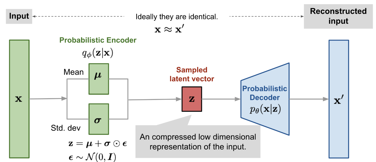
Figure 3: Illustration of Variational Autoencoder model
Understanding Each Term of the ELBO
| Term | Meaning | Analogy |
|---|---|---|
| $ \mathbb{E}{q_\phi}[\log p_\theta(x \mid z)]$ | Reconstruction accuracy | “How well can I rebuild the input?” |
| $ \mathrm{KL}(q_\phi(z \mid x) \Vert p(z))$ | Latent regularization | “How close are my latent codes to the ideal Gaussian?” |
A large KL means the model is overfitting per-sample latents.
A small KL (too close to 0) means the model is ignoring $z$ is a problem known as posterior collapse.
β-VAE (Beta Variational Autoencoder)
β-VAE (Higgins et al., 2017) is a modification of the Variational Autoencoder (VAE) designed to encourage disentangled latent representations. Disentanglement means that each dimension in the latent space corresponds to a distinct, interpretable generative factor, and is invariant to changes in other factors.
If each latent variable in the inferred representation is sensitive to only one generative factor and invariant to others, the representation is said to be disentangled or factorized. For example, a model trained on human face images may encode features such as skin color, hair length, or wearing glasses in separate latent dimensions. Such representations improve interpretability and generalization.
β-VAE Objective as a Constrained Optimization Problem
To promote disentanglement, β-VAE imposes a constraint on the latent information capacity:
\[\max_{\phi, \theta} \quad \mathbb{E}_{p(x)} \mathbb{E}_{q_\phi(z \mid x)}[\log p_\theta(x \mid z)]\]subject to
\[\mathbb{E}_{p(x)} \left[ \mathrm{KL}(q_\phi(z \mid x) \| p(z)) \right] \leq \epsilon\]where $ \epsilon > 0 $ limits the amount of information encoded in $ z $.
Lagrangian Formulation and KKT Conditions
Using the Karush–Kuhn–Tucker (KKT) conditions, this constrained problem can be converted to an unconstrained optimization via a Lagrange multiplier $ \beta \geq 0 $:
\[\mathcal{L}(\phi, \theta, \beta) = \mathbb{E}_{p(x)} \mathbb{E}_{q_\phi(z \mid x)}[\log p_\theta(x \mid z)] - \beta \left( \mathbb{E}_{p(x)} \left[ \mathrm{KL}(q_\phi(z \mid x) \| p(z)) \right] - \epsilon \right)\]Ignoring constants that don’t affect optimization, we get the β-VAE loss:
\[\boxed{ \mathcal{L}_{\beta\text{-VAE}}(\phi, \theta) = \mathbb{E}_{p(x)} \mathbb{E}_{q_\phi(z \mid x)}[\log p_\theta(x \mid z)]- \beta \cdot \mathbb{E}_{p(x)} \left[ \mathrm{KL}(q_\phi(z \mid x) \| p(z)) \right] }\]where
- $ \beta = 1 $ recovers the standard VAE
- $ \beta > 1 $ applies stronger bottleneck constraints
Interpretation
- The reconstruction term encourages the model to accurately reconstruct data.
- The KL term regularizes the encoder to produce latent codes close to the prior.
- Increasing $ \beta $ penalizes latent capacity, pushing the model to encode minimal but meaningful features.
- This encourages disentanglement because the model prefers independent latent factors to efficiently represent data.
Information Bottleneck Perspective
This aligns with the Information Bottleneck principle (Tishby et al., 2000), where we want to maximize relevant information retained and minimize irrelevant information:
\[\max_{q(z|x)} I(z; y) - \beta I(x; z)\]In unsupervised learning, since $ y $ is unavailable, the objective reduces to balancing reconstruction and compression, exactly what β-VAE achieves.
- Higher $ \beta $ leads to more factorized latents but worse reconstructions.
- Tuning $ \beta $ is essential depending on downstream tasks.
- Extensions such as β-TCVAE (Chen et al., 2018) further improve disentanglement by decomposing KL.
Vector-Quantized Variational Auto Encoder (VQ-VAE)
Traditional VAEs model a continuous latent space using Gaussian distributions, but this may not align well with the structure of discrete data. Vector-Quantized Variational Auto Encoder (VQ-VAE) (Van den Oord, et.al 2017) learns discrete latent variables.
VQ-VAE models learn such discrete embeddings using vector quantization. A method that’s closely related to k-nearest neighbors (KNN) clustering.
Let $\mathcal{E} \in \mathbb{R}^{K \times D}$ denote the codebook or latent embedding space, where:
- $K$ is the number of discrete embedding vectors
- $D$ is the dimensionality of each embedding
Each individual codebook vector is represented as $e_i \in \mathbb{R}^D$, for $i = 1, \dots, K$.
Given an input $x$, the encoder produces a latent representation: \(z_e = E(x)\)
This continuous representation is then quantized by performing a nearest-neighbor lookup in the codebook: \(e_k = \arg\min_{e_i \in \mathcal{E}} \|z_e - e_i\|_2\)
The selected code vector $e_k$ is passed to the decoder $D(\cdot)$ to reconstruct the output.
Discrete latent variables can have different shapes in differnet applications. For example, 1D for speech, 2D for image etc.
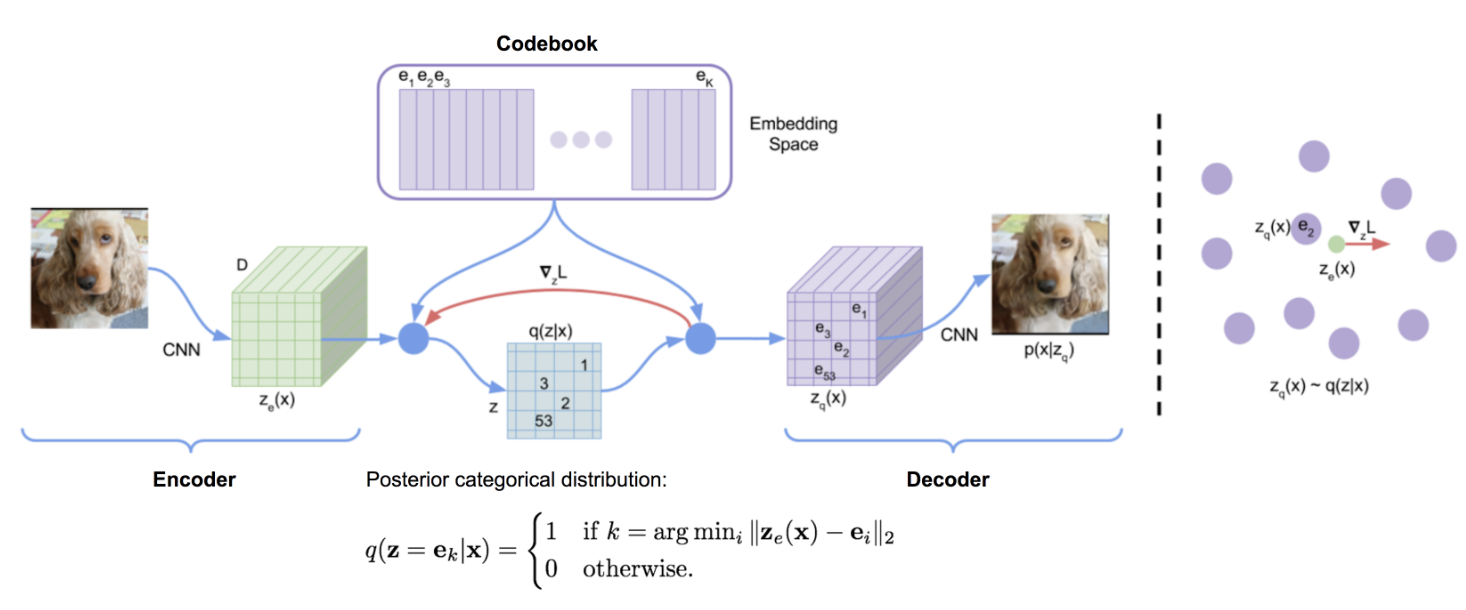
Figure 4: VQ-VAE architecture (source : Van den Oord, et.al 2017)
Handling non-Differentiable Quantization
The argmin is non-differentiable in discrete space. So, the VQ-VAE copies the gradients $\nabla{z_q}L$ from decoder input $z_e$ into encoder output $z_e$. mathematically :
\[z_q = sg[e_k] + (z_e - sg[z_e])\]Here, $sg[.]$ is stop gradient operator.
Loss Function
\[\mathcal{L} = \underbrace{\|x - \hat{x}\|_2^2}_{\text{Reconstruction}} + \underbrace{\| \text{sg}[z_e(x)] - e_k \|_2^2}_{\text{Codebook (VQ)}} + \underbrace{\beta \cdot \| z_e(x) - \text{sg}[e_k] \|_2^2}_{\text{Commitment loss}}\]The VQ loss updates the codebook embeddings (because $e_k$ receives gradients). Commitment loss updates the encoder $z_e$.
Updating the Codebook via EMA
Instead of training $ e_i $ via gradient descent (which may be unstable), VQ‑VAE uses Exponential Moving Average (EMA) updates.
For each code $ e_i $, we track:
- $ N_i $: the (smoothed) count of how many encoder outputs chose code $ i $
- $ m_i $: the (smoothed) sum of those encoder outputs that mapped to $ e_i $
At batch $ t $, the updates are defined as:
\[N_i^{(t)} = \gamma N_i^{(t-1)} + (1 - \gamma) \, n_i^{(t)}\] \[m_i^{(t)} = \gamma m_i^{(t-1)} + (1 - \gamma) \sum_{j=1}^{n_i^{(t)}} z_e^{(j)}\] \[e_i^{(t)} = \frac{m_i^{(t)}}{N_i^{(t)}}\]Where:
- $ \gamma \in [0, 1) $ is the EMA decay factor
- $ n_i^{(t)} $ is the number of encoder outputs in the current batch assigned to code $ e_i $
- $ z_e^{(j)} $ is the encoder output assigned to $ e_i $ in the current batch
This EMA-based approach ensures smooth and stable updates of the codebook entries.
References
- Carl Doersch, 2016. Tutorial on Variational Autoencoders
- Aaron van den Oord, et al., NIPS 2017. Neural Discrete Representation Learning
- Diederik P. Kingma, and Max Welling., ICLR 2014. Auto-encoding variational bayes.
- Weng, Lilian, lilianweng.github.io, 2018. From Autoencoder to Beta-VAE
- YouTube Tutorial: Variational AutoEncoders , Generative AI Animated
- YouTube Tutorial: Variational Autoencoders
- YouTube Tutorial: Understanding Variational AutoEncoders (VAEs)
- YouTube Tutorial: Vector-Euantized Variational AutoEncoders (VQ-VAEs)
- YouTube Tutorial: Variational Autoencoder - Model, ELBO, loss function and maths explained easily!
Citated as :
Sripadam, Sujith S. (Oct.2025)
From Autoencoder to VQ-VAE.
sujithsaisripadam.github.io/2025/10/17/vae/., 2025.
@article{sripadam2025VAE,
  title   = "From Autoencoder to Beta-VAE",
  author  = "Sripadam, Sujith S.",
  journal = "sujithsaisripadam.github.io",
  year    = "2025",
  url     = "https://sujithsaisripadam.github.io/2025/10/18/vae.html"
}